New ChainerMN functions for improved performance in cloud environments and performance testing results on AWS
ChainerMN is a package that adds multi-node distributed learning functionality to Chainer. We have added the following two new functions to v1.2.0 and v1.3.0 of ChainerMN, which are intended to improve the performance on systems whose inter-node communication bandwidth is low.
- Double buffering to conceal communication time
- All-Reduce function in half-precision floats (FP16)
It had previously been difficult to achieve high parallel performance in a system environment without a high-speed network because ChainerMN was developed assuming a supercomputer-like system with a high-speed network. With these newly-added functions, ChainerMN will be able to achieve high parallel performance even in the cloud and other common systems such as Amazon Web Services (AWS) as we presented at GTC2018.
Background
In data parallel distributed deep learning, the training time is typically dominated by the All-Reduce operation to calculate the sum gradients computed per node. We solved this issue on PFN’s 1,024 GPU supercomputer by utilizing high-speed InfiniBand interconnect, which is also used in supercomputers and Microsoft Azure, and also using the NVIDIA Collective Communications Library (NCCL) that enables fast execution of All-Reduce functions [1]. However, AWS and other commonly used systems have larger communication overhead because they do not have such a high-speed interconnect as InfiniBand. As a result of this, we could not make training faster simply by increasing the number of nodes in some cases. To solve these issues, we have added two function to ChainerMN v1.2.0 and v1.3.0: a double buffering function to conceal communication time and an All-Reduce function in FP16.
Function to conceal communication time by double buffering
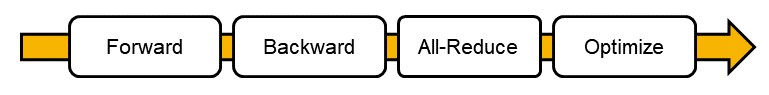
This function conceals the time it takes to communicate and shortens the overall computation time by having computation (forward, backward, and optimize) and communication (All-Reduce) processes overlapped. Normally in ChainerMN, one iteration consists of the four steps in the below diagram: forward, backward, All-Reduce, and optimize.
Using double buffering to conceal the communication time, the calculation and communication processes can overlap as in the below diagram.
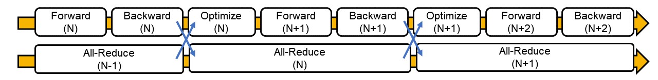
In this case, the optimization process is performed using gradients in the previous iteration. This means it uses old gradients to optimize the model, possibly affecting accuracy. We have learned, however, that almost the same level of accuracy can be maintained when training on ImageNet as demonstrated in the experiment described later in this article.
You can use this function just by making double_buffering=True when creating a multi-node optimizer as shown below.
optimizer = chainermn.create_multi_node_optimizer(optimizer, comm, double_buffering=True)
Currently, this function only supports the pure_nccl communicator.
All-Reduce function in FP16
ChainerMN v1.2.0 only supported All-Reduce in FP32 but v1.3.0 supports FP16 as well. This allows you to perform distributed training even for FP16 models using ChainerMN. We can expect a significant reduction in All-Reduce time by using FP16 because the communication volume is halved in comparison with using FP32. In addition, now you can use FP16 for only All-Reduce and reduce the All-Reduce time, even if you used FP32 in computation. This is the technique we employed for training on ImageNet using 1,024 GPUs [1].
For FP16 models, All-Reduce is carried out in FP16 without making any change. You can use different data types for computation and All-Reduce by putting allreduce_grad_dtype='float16' when creating a communicator as shown below.
comm = chainermn.create_communicator('pure_nccl', allreduce_grad_dtype='float16')
This function only supports the pure_nccl communicator as of today, as double buffering does likewise.
Results
To demonstrate high parallel performance using the two new functions, we measured performance using image classification datasets on ImageNet. We used ResNet-50 as the CNN model. In this experiment, we used 10Gb Ethernet of PFN’s supercomputer MN-1 and AWS as low-speed networks. For more details on the experiment setting, please refer to the appendix at the end of this article.
Evaluation using 10Gb Ethernet
The following graphs show changes in the throughput as the number of GPUs is increased in three cases using MN-1: Infiniband FDR, 10Gb Ethernet, and 10Gb Ethernet using the two new functions.
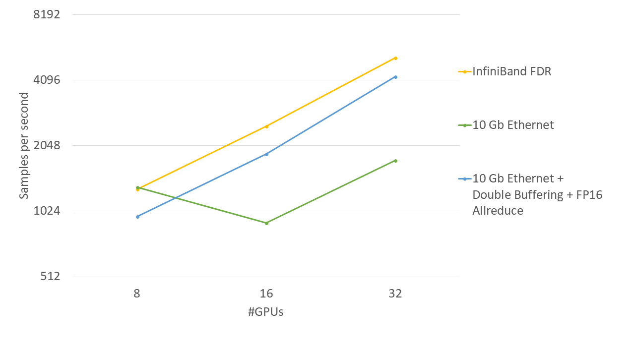
As you can see in the figure, the performance did not improve even as we increased the number of GPUs when using the 10Gb Ethernet while the use of the new functions enabled it to achieve the ideal speedup with the performance scaling linearly with the number of GPUs.
The following table also shows the average validation accuracy and average training hours when conducting training for five times with the number of epochs = 90 and 32 GPUs.
| Validation Accuracy (%) | ComputingTime (hour) | |
|---|---|---|
| InfiniBand FDR | 76.4 | 6.96 |
| 10 Gb Ethernet | 76.4 | 21.3 |
| 10 Gb Ethernet + Double Buffering + FP16 Allreduce | 75.8 | 7.71 |
As you can see, the two new functions had almost no impact on accuracy. In the meantime, it just took 11% longer to train the model when using the 10 Gb Ethernet and the new functions than when using Infiniband FDR. With this, we can conclude that high parallel performance can be achieved while maintaining the level of accuracy, without a need to use Infiniband or other high-speed networks.
Evaluation using AWS
In testing with AWS, we used p3.16xlarge. This instance has eight V100, which is the highest-performance GPU available as of May 2018. The following graphs show changes in the throughput as the number of GPUs increased when using this instance.
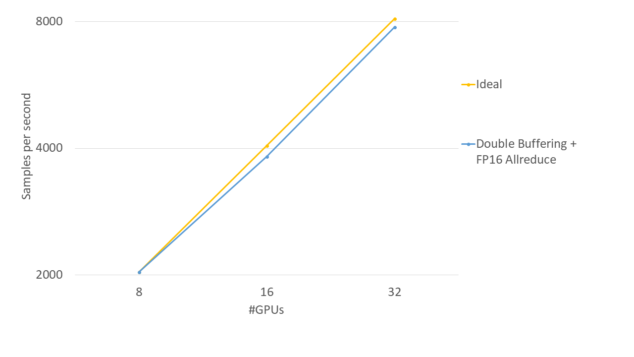
Scaling efficiency is an indicator often used to measure parallel performance. In this experiment, the scaling efficiency is expressed as \(e\) using the following equation where the base throughput is \(t_0\) and the throughput when \(n\) x base GPUs are used is \(t\).
\[e = t/(t_0*n)\]It indicates that the closer \(e\) gets to 1 (100%), the higher the parallel performance is. In this experiment, the scaling efficiency was 96% at 32GPUs when using 8GPUs as the base, demonstrating that the high parallel performance has been achieved by using the new functions.
Outlook for the future
We plan to add more functions to ChainerMN, including model parallelism to support various training models that are not achievable by data parallel as well as a function to improve fault tolerance. Our team is not only developing ChainerMN but also putting efforts into making Chainer and CuPy faster, and doing large-scale research and development activities by making the full use of MN-1, which is equipped with 1,024 P100 units, and the next-generation cluster with 512 V100 units. If you are interested in working with us on these activities, send us your application!
Appendix
Performance measurement details
Experiment setup
- Dataset:ImageNet-1k
- Model:ResNet-50 (input image size 224×224)
Setup for measuring throughputs
- Batch size:64
- Training rate:fixed
- Data augmentation:using the same method as Goyal et al. [2]
- Optimization:Momentum SGD (momentum=0.9)
- Weight decay: 0.0001
- # of measurements:400 iterations
Setting for training with # of epochs = 90
- Batch size:64 per GPU until the 30th epoch, 128 afterwards
- Training rate:Gradual warmup until the 5th epoch, 0.2 time at the 30th epoch, and 0.1 time at the 60th and 80th epochs.
- Data augmentation:using the same method as Goyal et al. [2]
- Optimization:Momentum SGD (momentum=0.9)
- Weight decay: 0.0001
- # of epochs:90 epochs
- In general, this setup is based on Goyal et al. [2] and uses the technique described in Smith et al. [3].
Experiment conditions in the verification test using 10Gb Ethernet
- Max 4 nodes, 32 GPUs in total
- Node
- GPU: 8 * NVIDIA Tesla P100 GPUs
- CPU: 2 * Intel Xeon E5-2667 processors (3.20 GHz, 8 cores)
- Network: InfiniBand FDR
- Save location for training data:local disk
Experiment conditions in the verification test using AWS
- Max 4 nodes, 32 GPUs in total
- Node(p3.16xlarge)
- GPU: 8 * NVIDIA Tesla V100 GPUs
- CPU: 64 vCPUs
- Network: 25 Gbps network
- Save location for training data:RAM disk
References
[1] Akiba, T., et al. Extremely Large Minibatch SGD: Training ResNet-50 on ImageNet in 15 Minutes. CoRR, abs/1711.04325, 2017.
[2] Goyal, P., et al. Accurate, Large Minibatch SGD: Training ImageNet in 1 Hour. CoRR, abs/1706.02677, 2017.
[3] Smith, S. L., et al. Don’t Decay the Learning Rate, Increase the Batch Size. CoRR, abs/1711.00489, 2017.
About Chainer
Chainer is a Python-based, standalone open source framework for deep learning models. Chainer provides a flexible, intuitive, and high performance means of implementing a full range of deep learning models, including state-of-the-art models such as recurrent neural networks and variational autoencoders.
Recent Posts
- Chainer/CuPy v7 release and Future of Chainer
- Chainer/CuPy v7のリリースと今後の開発体制について
- Sunsetting Python 2 Support
- Released Chainer/CuPy v6.0.0
- ChainerX Beta Release
- Released Chainer/CuPy v5.0.0
- ChainerMN on AWS with CloudFormation
- Open source deep learning framework Chainer officially supported by Amazon Web Services
Categories
- General (12)
- Announcement (10)